[AI Sparks] Issue 10: The Power of Many: The Hidden Brain

Welcome back to AI Sparks!

In our last issue, we built a Linear Classifier. It was our first neural network, but as we discussed, it was more of a "reflex" than a brain. It connected pixels directly to categories, drawing straight mathematical lines to make decisions. It hit a ceiling of about 85% accuracy because real-world data—like a folded shirt or a tilted sneaker—is too complex for straight lines.

Today, we go Deep.

We are going to give our model a "digital cortex" by adding a Hidden Layer. This is the moment we move from simple baseline model into the true world of Neural Networks. We will see the accuracy of our model increases as we teach it how to "bend" its logic to handle the beautiful complexity of the real world.

Inside this Issue:

• 📡 AI Radar: The Trillion-Parameter Era
• 💡 Concept Quick-Dive: Anatomy of a "Dense" Neural Network
• 🛠️ Hands-on Lab: Build Your First "Real" Neural Network
• 🧪 Experiment: Tweak the Network
• 💥 Capstone Challenge: Can You Read Hands?

📡 AI Radar: The Trillion-Parameter Era

What Happened?

In today’s hands-on lab, you will build a neural network by wiring 128 neurons together. This creates a web of about 100,000 parameters (the total count of weights and biases) to tune—making the model smart enough to recognize a shoe or a shirt in an image.

In the industry, however, we have left the "thousands" behind and entered the era of the Trillion-Parameter model. While exact specs are secret, industry analysis suggests that GPT-5 operates with roughly 1.8 trillion parameters. To handle this massive scale, it is rumored to use a "Mixture of Experts" (MoE) architecture—essentially a committee of 8 massive neural networks working together. Training a system this size is an engineering marvel that costs over $100 million for a single run.

Why It Matters:

For a long time, researchers thought that to get "smarter" AI, we needed new, more complex algorithms. But the biggest breakthrough of the last few years is the discovery of Scaling Laws.

It turns out that if we take the exact same architecture you are learning today—simple neurons, weights, and biases—and just make it massively larger while feeding it more data, "emergent behaviors" begin to appear. Suddenly, the model isn't just predicting the next word; it starts to reason, write code, and solve logic puzzles—skills it wasn't explicitly taught.

The "So What" for Students?

First, the fundamentals we are learning today from a small neural network—how to build a neural network, how to tune hyperparameters, or why a model overfits—are the absolute bedrock of models like GPT-5 and Gemini. You aren't learning a "beginner version" of AI that you'll have to unlearn later. You are learning the exact physics that powers the most advanced AI models on Earth. Master the small scale first, and you will understand the large scale.

Second, this highlights the next major skill for students to acquire: Engineering for Scale. While the math is the foundation, building and tuning massive neural networks on huge datasets requires a whole new set of "Pro" techniques. That is what separates a hobbyist from an AI Engineer.

💡 Concept Quick-Dive: Anatomy of a "Dense" Neural Network

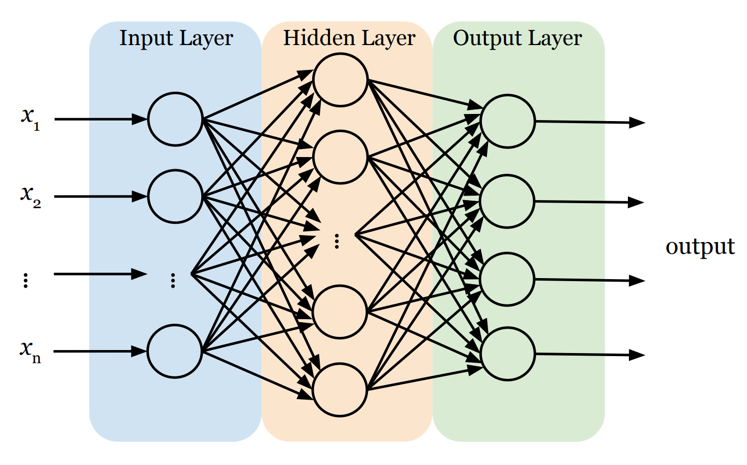
Before we start coding, let's understand the blueprint. In our lab, we will use an AI model often called a Dense Neural Network. It has three distinct parts:

1. The Input Layer (The Retina): This is the network's front door. Its only job is to receive raw data (i.e., features x₁ , x₂ , ..., x_n) and pass it on. Crucially, standard neural networks generally expect their input as a flat list (a vector). So, if the input is not a vector, we need to first convert it into one.
2. The Hidden Layers (The Brain): This is where the actual thinking happens. A neural network can have just one hidden layer or stack many of them deep. Sandwiched between input and output, these layers are responsible for finding patterns.

• Same Math, Larger Scale: Every single neuron in these layers works exactly like the one we built last time. It receives inputs, calculates a weighted sum, adds a bias, and feeds the result into an activation function.
• Fully Connected: In a "Dense" neural network, every single neuron in a hidden layer is connected to every single neuron in the previous layer. This web of connections allows the network to combine information in complex ways.
• Hierarchical Learning: Early layers act like detectives looking for simple clues, and deeper layers combine those clues to recognize complex patterns.
• ReLU Activation: In this issue, we will use the ReLU (Rectified Linear Unit) activation function instead of the Sigmoid function. Its math is incredibly simple: f(x) = max(0, x).
  • If the signal is negative (no pattern found), it outputs 0 (shuts the neuron up).
  • If the signal is positive, it passes it through.

This simple "on/off" switch allows the network to ignore irrelevant noise and focus only on the features that matter, creating a complex, "bent" boundary that can separate a shirt from a coat far more accurately than a straight line ever could.

3. The Output Layer (The Decision): This is the final verdict. The structure here is strict: we need exactly one neuron for every category we want to predict. We use a function called Softmax here, which forces each neuron to output a single score between 0 and 1, representing the probability that the current data sample belongs to its category. To make the final prediction, we simply pick the winner—the category with the highest score.

🛠️ Hands-on Lab: Build Your First "Real" Neural Network

In this lab, we will take the baseline model code from last issue and upgrade it with a "Hidden Brain."

💻 Getting Started: Setup & Tools

Open a new file in your Python IDE or Google Colab (recommended). We’ll need the following libraries:

• tensorflow / keras: To build and train the neural network.
• numpy: For handling the data arrays.
• matplotlib: To visualize the actual images.

📋 Instructions

Step 0: Load and Visualize the Data

We'll use Fashion-MNIST. Recall that this dataset consists of 70,000 grayscale images of 10 different clothing categories (60,000 for training and 10,000 for testing). Each image is 28×28 pixels, meaning it contains a total of 784 pixels. Every pixel has a single integer value ranging from 0 (black) to 255 (white), representing the brightness of that point. Hence, the computer sees each image not as a picture, but as a 28×28 array of integers. Additionally, each image is associated with a label, which is an integer from 0 to 9, representing the category of clothing (e.g., 0 is T-shirt, 9 is Ankle boot).

The following code loads the dataset and displays the first image in the training set.

import tensorflow as tf
from tensorflow import keras
import numpy as np
import matplotlib.pyplot as plt

# 1. Load the Fashion-MNIST dataset (built into Keras)
(train_images, train_labels), (test_images, test_labels) = keras.datasets.fashion_mnist.load_data()

# 2. Define the class names (so we see "Sneaker" instead of "7")
class_names = ['T-shirt/top', 'Trouser', 'Pullover', 'Dress', 'Coat',
               'Sandal', 'Shirt', 'Sneaker', 'Bag', 'Ankle boot']

# 3. Let's look at one!
plt.imshow(train_images[0], cmap='gray')
plt.title(f"Label: {class_names[train_labels[0]]}")
plt.show()

Step 1: Preprocess the Data

Data preprocessing is the essential step of cleaning and formatting raw data before feeding it into an AI model. In our case, we need to perform Normalization on the image data. The raw pixel values in our images range from 0 to 255. However, neural networks prefer small numbers (0-1) over large ones (0-255). By dividing our pixel values by 255.0, we scale the data down to a range between 0 and 1. This simple math trick makes training faster and more stable.

# Scale pixel values from [0, 255] to [0.0, 1.0]

train_images = train_images / 255.0
test_images = test_images / 255.0

Step 2: Build the Model

We will construct a neural network with three specific layers:

1. Input Layer: This is where we feed data into a neural network. Neural networks typically require input in the form of a vector (a simple list of numbers). Since our images are grids of 28×28 pixels, we will "flatten" them into a vector. We simply take the first row of pixels, attach the second row to the end of it, and repeat for all rows to form one single long line of 784 (=28×28) input values and feed them into the network.
2. Hidden Layer: This is the learning engine. We will use 128 neurons. Why 128? It's an arbitrary choice—large enough to learn complex patterns (like "shoe laces" or "sleeves") but small enough to run quickly on a laptop.
3. Output Layer: This is the decision maker. We must use exactly 10 neurons here because our dataset has 10 categories of clothing. Each neuron outputs a probability score. To make the final decision, we look at all 10 scores and pick the category with the highest probability.

model = keras.Sequential([
    keras.layers.Input(shape=(28, 28)),          # Define input shape
    keras.layers.Flatten(),                      # Flatten 28x28 to 784 pixels
    keras.layers.Dense(128, activation='relu'),  # Hidden layer (128 neurons)
    keras.layers.Dense(10, activation='softmax') # Output layer (10 classes)
])

• keras.layers.Dense(128, ...): Remember the neuron we built last time? This line creates a hidden layer containing 128 of those neurons. It is called a "Dense" layer because the neurons are fully connected, meaning that every neuron in this layer is wired to receive input from every single neuron in the previous layer (i.e., the input layer).
  • activation='relu': We use the ReLU activation function.

Step 3: Compile and Train the Model

To train a neural network, we need two steps: Configuration (Compiling) and Execution (Training).

1. Compile (Defining the Rules of Learning): This step configures the model for training. We will specify the following strategies:

• Optimizer: How will we adjust the weights and biases in each neuron to minimize errors?
• Loss Function: The mathematical formula used to calculate the error between the guess and the true label.
• Metrics: How will we evaluate the performance of the network? (What we care about.)

2. Train (The Learning Loop): This is where the actual training occurs. The final output of the fit() method is a trained model with optimized weights and biases that can recognize images with minimal error.

# Compile the model
model.compile(optimizer='adam',
              loss='sparse_categorical_crossentropy',
              metrics=['accuracy'])

# Train the model
# We feed it the images and the correct labels in the training set
training_results = model.fit(train_images, train_labels, epochs=5)

# Print the training accuracy
train_acc = training_results.history['accuracy'][-1]
print(f"Training Accuracy: {train_acc*100:.2f}%")

Step 4: Evaluate the Model

Now that the model has learned, we need to give it a final exam. We test it on the test dataset—the 10,000 images it has never seen before. This gives us an unbiased report card. If the model does well here, we know it has truly learned the patterns and hasn't just memorized the training images.

# Check accuracy on the test set
test_loss, test_acc = model.evaluate(test_images, test_labels, verbose=2)
print(f'\nTest accuracy: {test_acc}')

In the last issue, the accuracy of the baseline model was likely around 84-85%. With this single hidden layer, it can jump to 88-89%.

🧪 Experiment: Tweak the Network

In the lab above, we simply use 5 epochs and 128 neurons. But why? Next, you will act as the lead researcher. Let's change these "hyperparameters" to see how they affect the model's intelligence.