[AI Sparks] Issue 9: The Power of Many: The First Connection

Welcome back to AI Sparks!

In our last issue, we zoomed in to the microscopic level. We built the fundamental atom of artificial intelligence: The Neuron. We did the math by hand, tweaking weights and biases to make a simple decision. It was impressive, but a single neuron is limited. It can only make simple, binary choices. It can decide to accept or reject a job offer, but it crumbles when faced with the messy complexity of the real world—like recognizing a handwritten number in a digital image or driving a car in traffic.

Today, we unlock the power of the crowd. We are moving from biology to architecture. We will take that single neuron, clone it, and wire a team of them into an interconnected structure: a Neural Network. By connecting these neurons, we create an AI model that can understand complex patterns and shapes that no single node could ever grasp alone.

This is the moment we cross the threshold from "simple math" to Machine Learning. We are stepping into the era where code doesn't just compute—it comprehends. By the end of this issue, you won’t just be calculating numbers for a single neuron like in the last issue; you will have built a base neural network that can decipher the visual world.

Inside this Issue:

• 💡 Concept Quick-Dive: What is Machine Learning (ML)?
• 💡 Concept Quick-Dive: The "Baseline" Neural Network
• 🛠️ Hands-on Lab: Build Your "Baseline" Neural Network
• 🧪 Experiment: Normalization Test
• 👥 Community Spotlight: Industry Insight — Keras vs. PyTorch

💡 Concept Quick-Dive: What is Machine Learning (ML)?

(Note: If you are already familiar with the core concepts of ML and classification, feel free to skip ahead to the next section.)

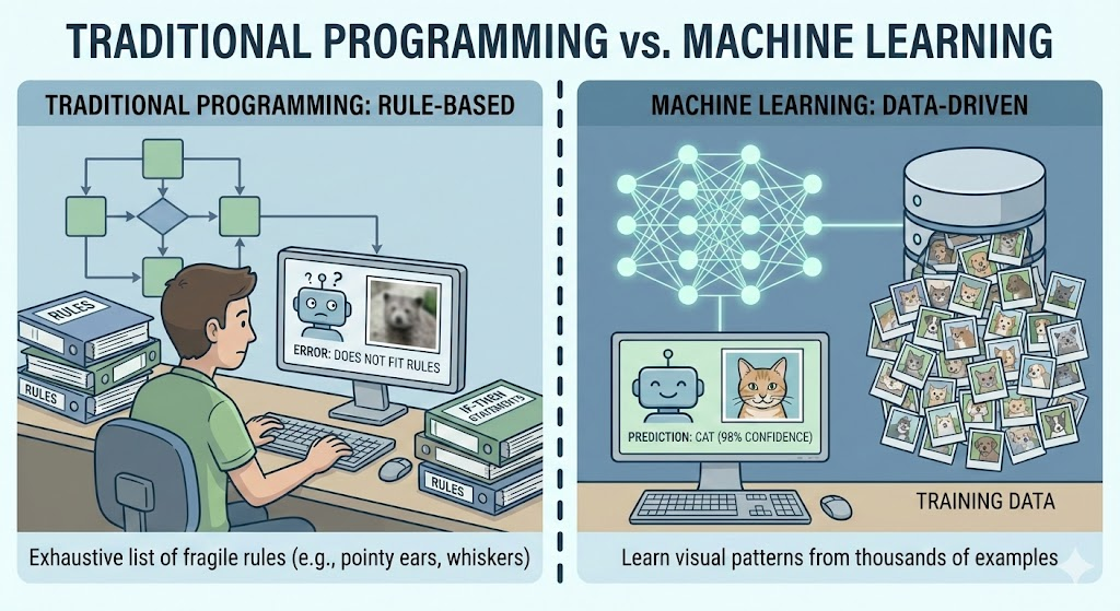
Machine Learning is a field of artificial intelligence where computers learn to make decisions or predictions by recognizing patterns in data, rather than following explicitly programmed instructions. To understand the difference, imagine we want to teach a computer to distinguish between photos of cats and dogs. In traditional programming, we would have to write an exhaustive list of strict rules (if image has pointy ears and whiskers and a small nose, then it is a cat), an approach that is incredibly fragile because real-world images are full of variations that rules cannot anticipate. In contrast, with machine learning, instead of writing rules, we show the computer thousands of photos of cats and dogs, allowing it to "learn" to distinguish between them by discovering the visual patterns that define each animal on its own.

What is Classification? Classification is one of the main flavors of machine learning where the goal is to predict a specific category, or "label," for a given piece of data. Consider a spam email filter: when a new message arrives, the system must decide if it belongs to "Spam" or "Not Spam." So, this is a classification problem. In this issue, we are performing Multi-class Classification. Instead of just two choices, we give the AI an image and it must choose the correct "bucket" out of 10 possible categories (Sneaker, Bag, Coat, etc.).

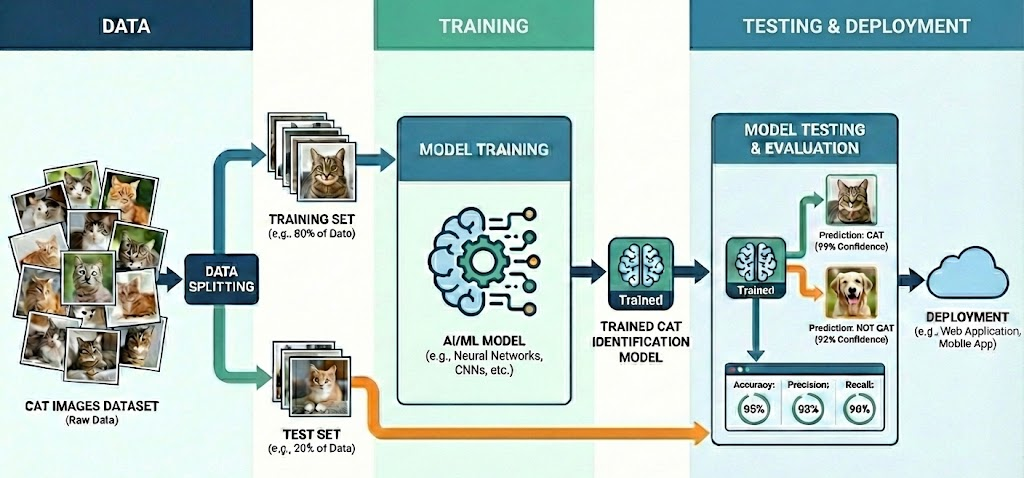
To bring a classification model to life, we follow a process that mirrors how humans learn. The heart of this journey is the Dataset, which consists of Features (the raw data inputs the computer analyzes) and Labels (the categories/labels we want the computer to predict). In image recognition, for example, the Features are the thousands of tiny pixels that make up the picture, while the Labels are the identities we assign them, like "Shirt" or "Bag." Once the data is ready, we begin Training, where the ML model examines the features, makes a guess, compares that guess to the true label, and tweaks its internal weights to get closer to the truth. Finally, we perform Testing, a "Final Exam" where we show the ML model data it has never seen before to evaluate its performance.

💡 Concept Quick-Dive: The "Baseline" Neural Network

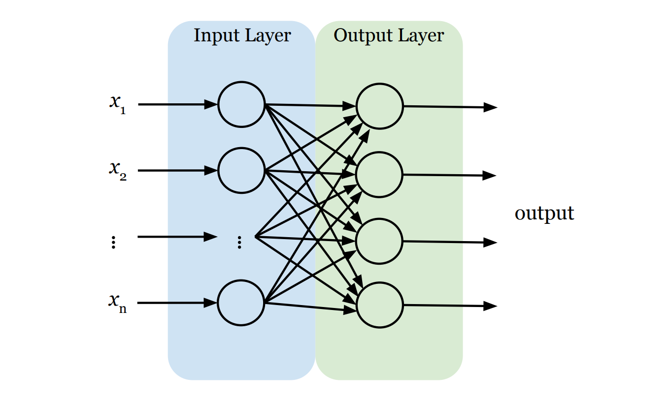
Because there is a lot of content to cover regarding neural networks, we have divided this topic into two issues. In this issue, we will build a "baseline" neural network. Think of this as a simplified, "starter" version of a neural network that connects inputs directly to outputs to establish a benchmark. In the next issue, we will move beyond this baseline to build a "real" neural network with added depth. For now, our baseline neural network model has exactly two layers:

1. The Input Layer (The Retina): This is the network's front door. Its only job is to receive raw data (i.e., features x₁ , x₂ , ..., x_n) and pass it on. Crucially, standard neural networks generally expect their input as a flat list (a vector). So, if the input is not a vector, we need to first convert it into one. For instance, if the input is an image, we first have to "flatten" that two-dimensional grid of pixels into a single, long line of numbers. The input layer doesn't think; it just takes raw data all in.
2. The Output Layer (The Decision): This is the final verdict. The structure here is strict: we need exactly one neuron for every category we want to predict. For example, if we are classifying clothes into 10 categories, we need 10 output neurons. Each output neuron is connected to every single feature from the input layer, ensuring the model considers the entire image before reaching a verdict. We use a function called Softmax here, which forces each neuron to output a single score between 0 and 1, representing the probability that the current data sample belongs to its category. The sum of all output scores equal exactly 100% (or 1.0). The result is like a confidence report: "I'm 90% sure this is a T-shirt, but there's a 10% chance it's a Coat." To make the final prediction, we simply pick the winner—the category with the highest score.

⚙️ The Engine Room: Thinking in Arrays

Before we start the lab, we need to introduce the tool we will use to handle data: NumPy (Numerical Python).

NumPy is the fundamental package for scientific computing in Python. It provides support for large, multi-dimensional arrays and matrices, along with a collection of high-level mathematical functions to operate on them. While Python lists are flexible, NumPy arrays are built for speed and efficiency, making them the industry standard for handling data in AI.

In AI and ML, we rarely work with single numbers. We work with Arrays (grids of numbers). For example, when working with image data, we often use 3-dimensional Arrays.

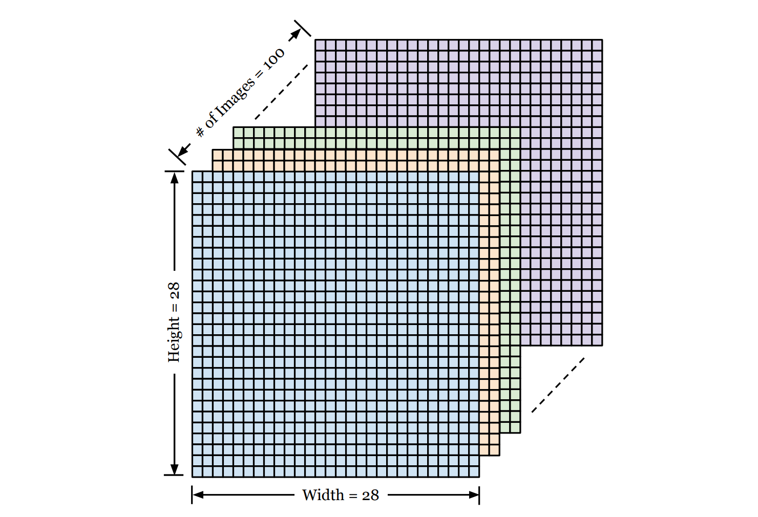
Imagine a stack of 100 images, each 28×28 pixels, we can use a 3-dimensional NumPy array of shape (100, 28, 28) to represent them, where

• Dimension 1: The number of images in the stack.
• Dimension 2: The height of each photo (in pixels).
• Dimension 3: The width of each photo (in pixels).

We can then use standard Python indexing to retrieve specific data from this stack (remember, indices start at 0):

• images[0] gives us the first image in the stack (a 28×28 grid).
• images[0][5][5] gives us the exact pixel value at row 5, column 5 of the first image.

We will use this structure heavily in the lab below!

🛠️ Hands-on Lab: Build Your "Baseline" Neural Network

In this lab, we are going to use a professional AI library called Keras to build a baseline neural network in just a few lines of code. By the end, you’ll have built and trained a neural network model that can scan images of clothing—from sneakers to shirts—and classify them instantly.

💻 Getting Started: Setup & Tools

Open a new file in your Python IDE or Google Colab (recommended). We’ll need the following libraries:

• tensorflow / keras: To build and train the neural network.
• numpy: For handling the data arrays.
• matplotlib: To visualize the actual images.

📋 Instructions

Step 0: Load and Visualize the Data

We'll use Fashion-MNIST, a popular dataset widely used for training and testing AI models. The dataset consists of 70,000 grayscale images of 10 different clothing categories (60,000 for training and 10,000 for testing). Each image is 28×28 pixels, meaning it contains a total of 784 pixels. Every pixel has a single integer value ranging from 0 (black) to 255 (white), representing the brightness of that point. Hence, the computer sees each image not as a picture, but as a 28×28 array of integers. Additionally, each image is associated with a label, which is an integer from 0 to 9, representing the category of clothing (e.g., 0 is T-shirt, 9 is Ankle boot).

The following code loads the dataset and displays the first image in the training set. Why visualize it? It's a crucial sanity check. Before asking an AI to learn, we always want to verify that the data loaded correctly and looks the way we expect. It helps us understand the "raw material" the network will be processing.

import tensorflow as tf
from tensorflow import keras
import numpy as np
import matplotlib.pyplot as plt

# 1. Load the Fashion-MNIST dataset (built into Keras)
(train_images, train_labels), (test_images, test_labels) = keras.datasets.fashion_mnist.load_data()

# 2. Define the class names (so we see "Sneaker" instead of "7")
class_names = ['T-shirt/top', 'Trouser', 'Pullover', 'Dress', 'Coat',
               'Sandal', 'Shirt', 'Sneaker', 'Bag', 'Ankle boot']

# 3. Let's look at one!
plt.imshow(train_images[0], cmap='gray')
plt.title(f"Label: {class_names[train_labels[0]]}")
plt.show()

Here is what each line does:

• import ...: We bring in our toolkit. tensorflow / keras is for building the brain, numpy for number crunching, and matplotlib for visualizing the images.
• keras.datasets.fashion_mnist.load_data(): Keras has this dataset built-in. This single line downloads the 70,000 images and automatically splits them into two piles: 60,000 images for training (learning the patterns) and 10,000 images for testing (evaluating performance). These are returned as four NumPy arrays with specific structures:
  • train_images: A 3-dimensional array of shape (60000, 28, 28). The first number (60,000) is the total count of images in the training set. The next two (28, 28) represent the height and width of each image in pixels.
  • train_labels: A 1-dimensional array where each element is an integer (0-9) representing the label for the corresponding image in the training set.
  • test_images: A 3-dimensional array of shape (10000, 28, 28) representing images in the test set.
  • test_labels: The 1-dimensional array of labels for the test set.
• class_names: The labels in the dataset are numerical (0-9), representing the 10 categories. This isn't very intuitive for us. We want to see human words. So we create this list with the human-readable names of the 10 categories. Later, we will use this list to translate a numerical label like "7" into a word label like "Sneaker."
• plt.imshow(...), plt.title(...), plt.show(): These commands work together to draw the image on the screen, add the correct label as a title, and finally display the plot so we can verify the data looks correct. train_images[0] grabs the first image in the training set, which gives us a 2-dimensional grid (28×28) of pixels representing the first shoe. We then draw this grid on the screen.

Step 1: Preprocess the Data

Data preprocessing is the essential step of cleaning and formatting raw data before feeding it into an AI model. Think of it like washing vegetables before cooking—raw data is often messy or in the wrong format for the "recipe."

In our case, we need to perform Normalization on the image data. The raw pixel values in our images range from 0 to 255. However, neural networks prefer small numbers (0-1) over large ones (0-255). By dividing our pixel values by 255.0, we scale the data down to a range between 0 and 1. This simple math trick makes training faster and more stable.

# Scale pixel values from [0, 255] to [0.0, 1.0]

train_images = train_images / 255.0
test_images = test_images / 255.0

When we write train_images / 255.0, it divides every single number inside the 3-dimensional array train_images by 255.0 at once.

Step 2: Build the "Baseline" Model

This is where the magic happens. Before writing the code, let's design the blueprint for our baseline neural network model. The model has exactly two layers:

1. Input Layer: This is where we feed data into a neural network. Neural networks typically require input in the form of a vector (a simple list of numbers). Since our images are grids of 28×28 pixels, we will "flatten" them into a vector. We simply take the first row of pixels, attach the second row to the end of it, and repeat for all rows to form one single long line of 784 (=28×28) input values and feed them into the network.
2. Output Layer: This is the decision maker. We must use exactly 10 neurons here because our dataset has 10 categories of clothing. Each neuron outputs a probability score. To make the final decision, we look at all 10 scores and pick the category with the highest probability.

model = keras.Sequential([
    keras.layers.Input(shape=(28, 28)),          # Define input shape
    keras.layers.Flatten(),                      # Flatten 28x28 to 784 pixels
    keras.layers.Dense(10, activation='softmax') # Output layer (10 classes)
])

• keras.Sequential(...): This creates a simple "stack" of layers, where data flows from the first layer to the last sequentially.
• keras.layers.Input(shape=(28, 28)): This explicitly tell the network the input is a 2-dimensional array of size 28×28.
• keras.layers.Flatten(): This transforms the format of an images from a 2-dimensional array (of 28×28 pixels) to a 1-dimensional array (of 784 pixels).
• keras.layers.Dense(10, ...): This creates the output layer with 10 neurons.
  • activation='softmax': The softmax function forces each neuron to output a probability score that sums to 100% (or 1.0).

Step 3: Compile and Train the Model

To train the baseline neural network, we need two steps: Configuration (Compiling) and Execution (Training).

1. Compile (Defining the Rules of Learning): This step configures the model for training. We will specify the following strategies:

• Optimizer: How will we adjust the weights and biases in each neuron to minimize errors?
• Loss Function: The mathematical formula used to calculate the error between the guess and the true label.
• Metrics: How will we evaluate the performance of the network? (What we care about.)

2. Train (The Learning Loop): This is where the actual training occurs. When we call the fit() method, the network enters a loop:

1. Forward Pass: It looks at each training image and makes a guess using its current weights and biases.
2. Calculate Error: It compares its guess to the true label to calculate the error.
3. Backward Pass (Backpropagation): It mathematically tweaks the weights and biases of every neuron to reduce that error.
4. Repeat: It does this thousands of times. The final output is a trained model with optimized weights and biases that can recognize images with minimal error.

# Compile the model
model.compile(optimizer='adam',
              loss='sparse_categorical_crossentropy',
              metrics=['accuracy'])

# Train the model
# We feed it the images and the correct labels in the training set
training_results = model.fit(train_images, train_labels, epochs=5)

# Print the training accuracy
train_acc = training_results.history['accuracy'][-1]
print(f"Training Accuracy: {train_acc*100:.2f}%")

• model.compile(...): This command locks in our configuration (optimizer, loss function, metrics) so the model is ready for training.
  • optimizer='adam': This specifies the optimization algorithm. We chose 'adam' because it is widely considered the best "all-purpose" optimizer for modern deep learning. Think of it as a smart coach that adjusts the learning speed automatically.
  • loss='sparse_categorical_crossentropy': This specifies the loss function. We chose Sparse Categorical Crossentropy because it is the standard method for classification tasks where labels are integers (like our 0-9 categories).
  • metrics=['accuracy']: This specifies the performance metric. We chose accuracy because it provides a clear, human-readable result: the percentage of images that the model classifies correctly.
• training_results = model.fit(...): This command starts the training loop.
  • epochs=5: One epoch is one full pass through the entire training set. Setting this to 5 means the network will review the entire set of 60,000 images 5 times to learn the patterns.
  • Once the training is completed, model.fit() returns a "Report Card" containing all the scores from the training process. We store this in the variable training_results.
• training_results.history['accuracy'][-1]: This command digs into the "Report Card" stored in the variable training_results to find the training accuracy we need.
  • .history: This accesses a dictionary called history inside training_results. It stores the results—such as training error and training accuracy—as key-value pairs.
  • ['accuracy']: This uses "accuracy" as the key to access the corresponding value in the history dictionary, which is a list of training accuracies recorded at the end of each epoch. It returns a list like [0.75, 0.8, 0.85, 0.88, 0.9].
  • [-1]: Grabs the last item in that list, representing the final training accuracy after the training finished.

Step 4: Evaluate the Model

Now that the model has learned, we need to give it a final exam. We test it on the test dataset—the 10,000 images it has never seen before. This gives us an unbiased report card. If the model does well here, we know it has truly learned the patterns and hasn't just memorized the training images.

# Check accuracy on the test set
test_loss, test_acc = model.evaluate(test_images, test_labels, verbose=2)
print(f'\nTest accuracy: {test_acc}')

• model.evaluate(...): This runs the model on the test data and returns two values: the loss and the accuracy.
  • test_loss: This is the mathematical error score on the test data (lower is better).
  • test_acc: This is the accuracy percentage on the test data (higher is better).
  • verbose=2: This parameter simply controls how much information is printed to the screen during the process. Setting it to 2 gives us a concise, one-line summary.

Step 5: Make Predictions

This is where we put the model to work in the real world. We give it a single new image, and it outputs a probability score for each of the 10 categories. We pick the category with the highest probability score as the final prediction result for the image.

In the following example, we will look at the prediction on the first image in the test set.

# Make predictions on all images in the test set
predictions = model.predict(test_images)

# Let's look at the prediction on the first image
predicted_label = np.argmax(predictions[0]) # Get the index of the highest confidence
true_label = test_labels[0]

print(f"Model predicts: {class_names[predicted_label]}")
print(f"Actual label:   {class_names[true_label]}")

# Show the image to verify
plt.imshow(test_images[0], cmap='gray')
plt.show()

• model.predict(test_images): This makes predictions for all the images in the test set. Note that for one image, it returns a list of 10 numbers (i.e., probability scores), not a single label.
• predictions[0]: We are accessing the prediction results for the first image in the test set, which is a list of 10 probability scores.
• np.argmax(...): This function is a helper from the NumPy library. It looks at the list of 10 probabilities and finds the index of the highest one. For instance, if the highest probability is in position 9 (Ankle boot), argmax returns 9, which is the predicted label for this image.
• class_names[...]: We use our translation list from Step 0 to convert that number (e.g., 9) back into a human word (e.g., "Ankle boot").

🧪 Experiment: Normalization Test

What happens if we forget to divide pixel values by 255.0?